Segmentation on CAD-PE Dataset.
The segmentation is performed on CAD-PE dataset
CAD-PE Segmentation
Unveiling Insights
Welcome to our blog, where we delve into the fascinating world of segmentation. The segmentation is performed on CAD-PE Challenge dataset "computer-aided design(CAD)", the precision and efficent segementation plays a pivotal role.
In this blog series
Please note that this blog and the work presented herein are the efforts of a beginner in the field of image processing. While every attempt has been made to ensure accuracy and provide valuable insights, there may be certain limitations or areas for improvement. If any inconveniences or shortcomings are encountered, I kindly request your understanding and forgiveness. This blog serves as a starting point for exploring the fascinating world of Image processing and computer vision, and I am eager to learn and grow from this experience. Your feedback and suggestions are greatly appreciated as they will contribute to my growth as a learner and researcher. Thank you for your support and understanding.
Join me as we unravel the complexities of segmentation on CAD-PE dataset, empowering you to leverage this knowledge in your research, industry projects, or even personal endeavours. So, fasten your seatbelts and get ready to explore the world of segmentation like never before!!.Let’s unlock the hidden potential within Deep learning models and unleash their power.


CAD-PE Dataset
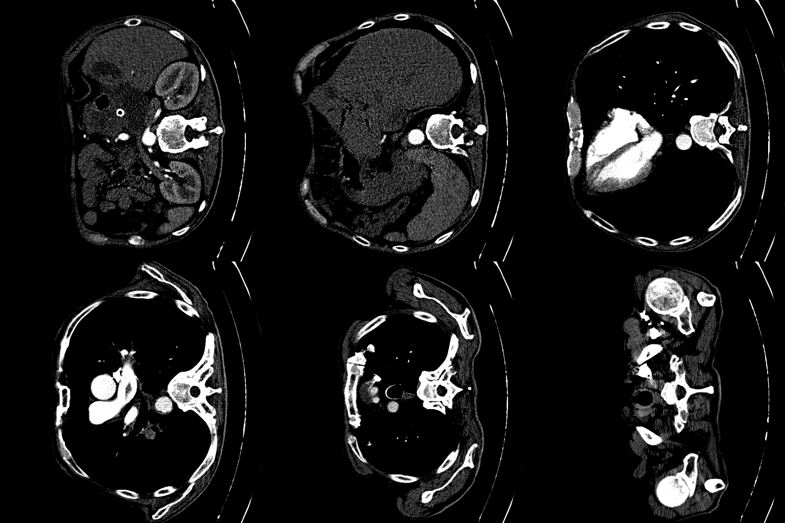
The first step involved is exploring the dataset. The dataset involves 91 patients CT scans. Each CT scan consists of some around 400 to 500 slices on average. Dividing the CT scans of the 91 patients into individual slices. This process allowed us to extract 41,256 slices in total, which will serve as the foundation for our segmentation endeavors.
Each slice within the CAD-PE dataset represents a two-dimensional image capturing a specific cross-section of the patients’ anatomy. These slices provide crucial insights into the internal structures and organs, enabling medical professionals and researchers to diagnose and study various conditions and diseases.
Building the Segmentation Dataset
Slice-Level Segmentation
In order to perform slice-level segmentation on the CAD-PE dataset, we will create a custom dataset named “segmentation_dataset”. This dataset will serve as the foundation for training and evaluating our segmentation algorithms.
To begin, we will divide the available data randomly into three sets: training, validation, and testing. The training set will contain 80% of the data, while the validation and testing sets will each consist of 10% of the data. This division ensures a balanced distribution of slices across the different sets, enabling us to train and assess the performance of our models effectively.
To handle the dataset efficiently, we will utilize filepaths to access the slices. Each slice within the CAD-PE dataset will be normalized to have pixel values ranging between 0 and 1. This normalization step ensures consistency and facilitates optimal model performance during training.
Moreover, the input images and corresponding segmentation masks will be processed to adhere to the requirements of slice-level segmentation. The input images will be converted into single-channel representations, while the segmentation masks will be transformed into binary masks, consisting of only 0s and 1s. These binary masks serve as ground truth annotations for the presence or absence of the target structures within the slices.
To facilitate seamless integration with deep learning frameworks, such as PyTorch, the slices will be transformed into tensors.
The snippet code provided below showcases a high-level implementation for building the segmentation_dataset:
class segmentation_dataset(Dataset):
def **init**(self,image_filenames,mask_filenames,transforms=None):
self.image_dir = "/CAD_PE_Challenge_Data/images/"
self.mask_dir = "/CAD_PE_Challenge_Data/masks/"
self.transform = transforms
self.image_filenames = image_filenames
self.mask_filenames = mask_filenames

def **len**(self):
return len(self.image_filenames)

def **getitem**(self, idx):
img = np.load(os.path.join(self.image_dir, self.image_filenames[idx]))
label = np.load(os.path.join(self.mask_dir, self.mask_filenames[idx]))

      img = nor_image(img)
      label = binary(label)
      if self.transform is not None:
          img, label = self.transform(img), self.transform(label)

      return img, label
Model Architecture of UNET
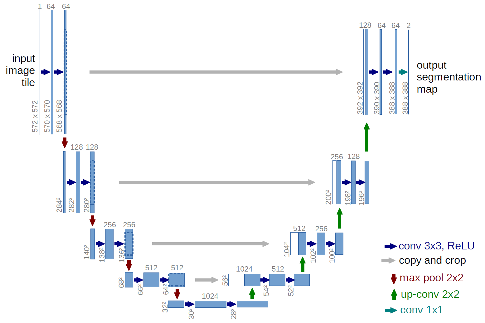
To perform slice-level segmentation on the CAD-PE dataset, we will utilize the UNet model
UNet model combines the prinicple of convolutional neural networks(CNNs) and has encoder-decodr architecture. The encoder design allows the model to effectively capture features (What? in the image) and decoder desgin allows the model to upsample the features and recover the spatial resolution (Where? in the image). Skip connections are incorporated to bridge the gap between the contracting and expanding paths, facilitating the propagation of low-level and high-level features.

Training the model
In the quest for accurate segmentation masks on the CAD-PE dataset, training a model becomes a crucial step. Leveraging the advancements in deep learning, we can harness the power of neural networks to tackle the challenging task of CAD-PE segmentation.
To begin the training process, we will employ the binary cross entropy with logits as the loss function. This loss function is particularly suited for segmentation tasks, as it compares the predicted segmentation masks with the ground truth masks, encouraging the model to accurately classify each pixel as belonging to the target structure or not.
For optimization, we will utilize the Adam optimizer, a popular choice for training deep learning models. With a learning rate of 0.001, the Adam optimizer dynamically adjusts the learning rate during training, optimizing the model’s performance and convergence.
To evaluate the quality of the segmentation results, we will employ the Dice coefficient as the evaluation metric. The Dice coefficient measures the overlap between the predicted and ground truth segmentation masks, providing a quantitative assessment of the model’s performance. A higher Dice coefficient indicates a better segmentation result, with values ranging from 0 (no overlap) to 1 (perfect overlap).
During the training process, the model will iteratively learn from the CAD-PE dataset, updating its parameters to minimize the loss function. By iteratively feeding the input slices and corresponding ground truth masks to the model, it will gradually learn to accurately segment the structures of interest.
The code snippet provided below showcases a high-level implementation for training the model for CAD-PE segmentation:
def train(epochs,model,train_loader,val_loader):

    #Define the loss function,optimizer, dice metric.
    loss_fn = nn.BCEWithLogitsLoss()
    optimizer = torch.optim.Adam(model.parameters(),lr = 0.001)
    dice = Dice(average='micro').to(device)

    train_loss = []
    val_loss = []
    avg_test_loss = []
    avg_dice = []
    avg_dice_val = []

    for epoch in tqdm(range(epochs)):
        model.train()
        # Training on Training set
        for i, (image, label) in enumerate(train_loader):

            image, label = image, label
            image, label = image.to(device), label.to(device)

            optimizer.zero_grad()
            output = model(image)
            loss = loss_fn(output, label)
            label = label.to(torch.int64)

            train_dice = dice(output, label)


            loss.backward()
            optimizer.step()

            train_loss.append(loss.item())
            avg_dice.append(train_dice.item())


        # evaluate on validation set
        model.eval()
        with torch.no_grad():
            for i, (image, label) in enumerate(val_loader):
                image, label = image, label

                image, label = image.to(device), label.to(device)

                output = model(image)
                loss = loss_fn(output, label)
                label = label.to(torch.int64)
                val_dice = dice(output, label)

                val_loss.append(loss.item())
                avg_dice_val.append(val_dice.item())

            val_loss_epoch = sum(val_loss) / len(val_loss)
            avg_dice_val_epoch = sum(avg_dice_val) / len(avg_dice_val)


        train_loss_epoch = sum(train_loss) / len(train_loss)
        avg_dice_epoch = sum(avg_dice) / len(avg_dice)

        # print average losses and dice coefficients for the epoch

        print(f"Epoch {epoch+1} | Train Loss: {train_loss_epoch:.5f} | Val Loss: {val_loss_epoch:.5f} |Dice Coefficient: {avg_dice_epoch:.5f} | Val Dice Coefficient: {avg_dice_val_epoch:.5f}")
By following this training process, we unlock the potential of deep learning to achieve accurate and reliable segmentation on the CAD-PE dataset. The model progressively learns to differentiate and classify the structures of interest.
Evaluating the Results
After training the UNet model on the CAD-PE dataset, it is time to evaluate the achieved results. The Dice coefficient, a widely used metric for segmentation tasks, provides a quantitative measure of the model’s performance.
On the training set, after training for 30 epochs, the UNet model achieved an impressive Dice coefficient of 0.88197. This indicates a significant overlap between the predicted segmentation masks and the ground truth masks, highlighting the model’s ability to accurately capture the target structures within the CAD-PE slices.
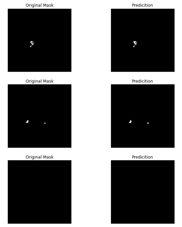
To further assess the generalization capability of the model, it is essential to evaluate its performance on the test set. On the test set, the UNet model attained a Dice coefficient of 0.70431. Although slightly lower than the training set performance, it still demonstrates the model’s effectiveness in accurately segmenting the target structures in previously unseen data.
To improve the model’s performance, several avenues can be explored. Firstly, hyperparameter tuning can be conducted by adjusting parameters such as learning rate, batch size, and regularization techniques. Fine-tuning these hyperparameters can potentially lead to better segmentation results.
Additionally, data augmentation techniques can be employed to augment the training set. Techniques such as random rotations, translations, and scaling can increase the diversity of the training data, enhancing the model’s ability to generalize to unseen samples.
Visualizing the model’s performance, the predicted segmentation masks can be compared side-by-side with the original ground truth masks.

Overall, the results achieved by the UNet model showcase its potential in CAD-PE segmentation. With further experimentation, fine-tuning of hyperparameters, and augmentation of the training data, it is possible to unlock even better segmentation results. The UNet model serves as a foundation for future advancements in segmentation.